Mean Reversion Trading Strategy Based on Moving Average

Pine ScriptMean reversion Trend following Volatility SMA

Author: ChaoZhang
Complexity: Intermediate · 135 lines
Parameters: 7
Backtest bar: 1d · swing
Tested on: BTC/USDT · futures

Jump to code View in vault Original on FMZ

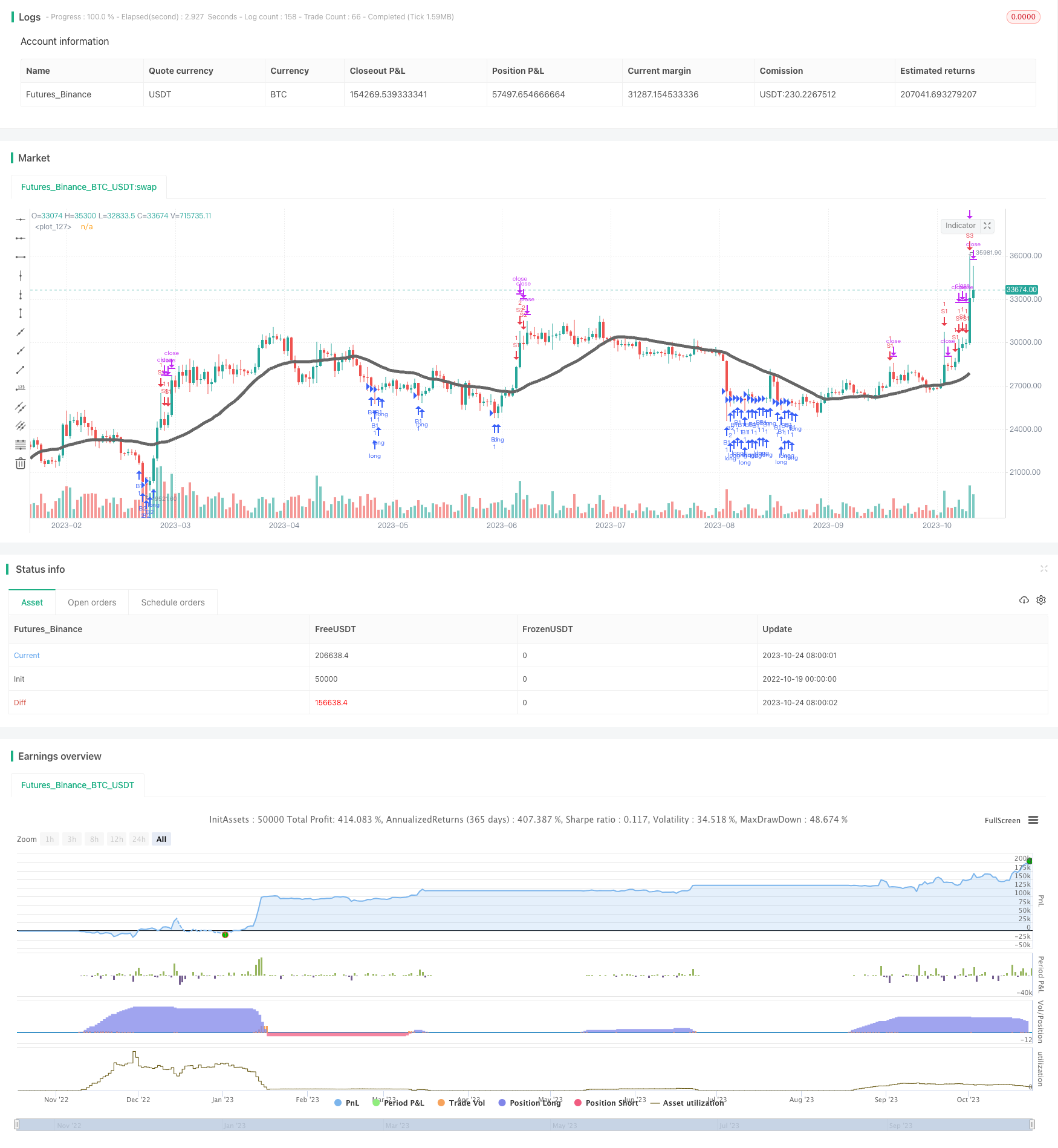
Overview

The mean reversion trading strategy is based on the price deviation from a moving average to make trading decisions. It takes advantage of the short-term deviation and long-term reversion pattern of prices to the mean by establishing positions when prices significantly below or above the moving average and closing positions when prices revert back.

Strategy Logic

The strategy first calculates a moving average over a certain period to represent the long-term price trend. Then it determines the timing and size of positions based on the deviation of price from the moving average.

When the price falls below the moving average by a certain percentage, it signals the price deviates from the long-term trend. In this case, long positions are gradually built with increasing size as the deviation widens. When the price bounces back above the moving average, suggesting a reversion to the mean, the long positions are closed for profit taking.

Similarly, when the price rises above the moving average by a threshold, short positions are built. When the price drops back towards the moving average, the short positions are closed with profits.

Advantage Analysis

Utilize the trend identification ability of moving averages to follow the long-term equilibrium trend of stock prices and identify the major trend direction.
Lower the average cost by scaling into positions, obtaining better entry prices.
Adopt staged take-profit to secure profits at different levels of mean reversion, lowering risks.
Control position sizing by fixed percentage to limit single trade loss size.
Flexible parameter settings such as moving average period and position sizing depending on different products.

Risk Analysis

Frequent stop loss when prices oscillate. Can widen stop loss range or add other filters.
Strong trend may break through moving average, unable to close at mean reversion. Can reduce position size identified by trend strength indicators.
Improper parameter settings may result in over-aggressive entries or stops. Cautious backtesting and adjustment based on market conditions are necessary.
High trading frequency leads to substantial trading costs. Cost factors should be considered in parameter optimization.

Improvement Directions

Optimize moving average period to adapt to product characteristics.
Optimize position sizing to balance risk and return.
Add other technical filters to avoid unnecessary trades.
Incorporate volatility measures to adjust position size based on market fluctuation levels.
Introduce profit target scaling to lower risk and increase return.

Conclusion

The mean reversion strategy utilizes the equilibrium reversion tendency of stocks by entering on deviation from the moving average and taking profit on reversion. With proper parameter tuning and filters, it can adapt to market changes and achieve good returns under risk control. The strategy incorporates both trend following and risk management, making it worth researching and applying for investors.

Parameters

Name	Default	What it controls
v_input_1	28	Moving Average (bars)
v_input_2	5	Deviation Increment (%)
v_input_3	true	Level 1 (units)
v_input_4	2	Level 2 (units)
v_input_5	4	Level 3 (units)
v_input_6	8	Level 4 (units)
v_input_7	16	Level 5 (units)

Source Pine Script

/*backtest
start: 2022-10-19 00:00:00
end: 2023-10-25 00:00:00
period: 1d
basePeriod: 1h
exchanges: [{"eid":"Futures_Binance","currency":"BTC_USDT"}]
*/

//@version=4
strategy("YJ Mean Reversion", overlay=true)
//Was designed firstly to work on an index like the S&P 500 , which over time tends to go up in value. 
//Avoid trading too frequently (e.g. Daily, Weekly), to avoid getting eaten by fees. 
//If you change the underlying asset, or time frame, tweaking the moving average may be necessary. 
//Can work with a starting capital of just $1000, optimise the settings as necessary. 
//Accepts floating point values for the amount of units to purchase (e.g. Bitcoin ). 
//If price of units exceeds available capital, script will cancel the buy. 
//Adjusted the input parameters to be more intuitive.

//input variables
movingAverage = input(title="Moving Average (bars)", type=input.integer, defval=28, minval=1, maxval=1000)
//riskPercentage = input(title="Amount to Risk (%)", type=input.integer, defval=1, minval=1, maxval=50)
deviation = input(title="Deviation Increment (%)", type=input.float, defval=5, minval=0.01, maxval=100) / 100
unitsLevel1 = input(title="Level 1 (units)", type=input.float, defval=1, minval=0.0001, maxval=10000)
unitsLevel2 = input(title="Level 2 (units)", type=input.float, defval=2, minval=0.0001, maxval=10000)
unitsLevel3 = input(title="Level 3 (units)", type=input.float, defval=4, minval=0.0001, maxval=10000)
unitsLevel4 = input(title="Level 4 (units)", type=input.float, defval=8, minval=0.0001, maxval=10000)
unitsLevel5 = input(title="Level 5 (units)", type=input.float, defval=16, minval=0.0001, maxval=10000)

//moving average and ma slope (use on weekly chart)
ma = sma(close, movingAverage)
//sl = ma > ma[4]

//units to buy
//amount = riskPercentage / 100 * (strategy.initial_capital + strategy.netprofit)
//units = floor(amount / close)

//mode 1
//strategy.order("buy", true, 1, when = (close < 0.95 * ma) and (strategy.position_size < 10))
//strategy.order("sell", false, strategy.position_size, when = (close > 1.05 * ma) and (strategy.position_size > 0))

//mode 2
//strategy.order("buy", true, 1, when = close < 0.8 * ma)
//strategy.order("sell", false, strategy.position_size, when = (close > 310) and (strategy.position_size > 0))

//mode 3
//strategy.order("buy", true, 1, when = (close < 0.95 * ma) and (close > 0.9 * ma))
//strategy.order("buy", true, 2, when = (close < 0.9 * ma) and (close > 0.85 * ma))
//strategy.order("buy", true, 4, when = (close < 0.85 * ma) and (close > 0.8 * ma))
//strategy.order("buy", true, 8, when = (close < 0.8 * ma) and (close > 0.75 * ma))
//strategy.order("buy", true, 16, when = (close < 0.75 * ma))
//strategy.order("sell", false, strategy.position_size, when = (close > 310) and (strategy.position_size > 0))

//mode 4
//strategy.order("buy", true, 1, when = (close < 0.98 * ma) and (close > 0.96 * ma) and (sl))
//strategy.order("buy", true, 2, when = (close < 0.96 * ma) and (close > 0.94 * ma) and (sl))
//strategy.order("buy", true, 4, when = (close < 0.94 * ma) and (close > 0.92 * ma) and (sl))
//strategy.order("buy", true, 8, when = (close < 0.92 * ma) and (close > 0.90 * ma) and (sl))
//strategy.order("buy", true, 16, when = (close < 0.90 * ma) and (sl))
//strategy.order("sell", false, strategy.position_size, when = (close > 310) and (strategy.position_size > 0))

//mode 5
//strategy.order("buy", true, 1, when = (close < 0.95 * ma) and (close > 0.9 * ma))
//strategy.order("buy", true, 2, when = (close < 0.9 * ma) and (close > 0.85 * ma))
//strategy.order("buy", true, 4, when = (close < 0.85 * ma) and (close > 0.8 * ma))
//strategy.order("buy", true, 8, when = (close < 0.8 * ma) and (close > 0.75 * ma))
//strategy.order("buy", true, 16, when = (close < 0.75 * ma))

//strategy.order("sell", false, 1, when = (close > 1.05 * ma) and (close < 1.1 * ma) and (strategy.position_size > 0))
//strategy.order("sell", false, 2, when = (close > 1.1 * ma) and (close < 1.15 * ma) and (strategy.position_size > 0))
//strategy.order("sell", false, 4, when = (close > 1.15 * ma) and (close < 1.2 * ma) and (strategy.position_size > 0))
//strategy.order("sell", false, 8, when = (close > 1.2 * ma) and (close < 1.25 * ma) and (strategy.position_size > 0))
//strategy.order("sell", false, 16, when = (close > 1.25 * ma) and (close < 1.3 * ma) and (strategy.position_size > 0))

//mode 6
//strategy.order("B1", true, unitsLevel1 * units, when = (close < 0.95 * ma) and (close > 0.9 * ma))
//strategy.order("B2", true, unitsLevel2 * units, when = (close < 0.9 * ma) and (close > 0.85 * ma))
//strategy.order("B3", true, unitsLevel3 * units, when = (close < 0.85 * ma) and (close > 0.8 * ma))
//strategy.order("B4", true, unitsLevel4 * units, when = (close < 0.8 * ma) and (close > 0.75 * ma))
//strategy.order("B5", true, unitsLevel5 * units, when = (close < 0.75 * ma))

//strategy.order("S1", false, unitsLevel1 * units, when = (close > 1.05 * ma) and (close < 1.1 * ma) and (strategy.position_size > 0))
//strategy.order("S2", false, unitsLevel2 * units, when = (close > 1.1 * ma) and (close < 1.15 * ma) and (strategy.position_size > 0))
//strategy.order("S3", false, unitsLevel3 * units, when = (close > 1.15 * ma) and (close < 1.2 * ma) and (strategy.position_size > 0))
//strategy.order("S4", false, unitsLevel4 * units, when = (close > 1.2 * ma) and (close < 1.25 * ma) and (strategy.position_size > 0))
//strategy.order("S5", false, unitsLevel5 * units, when = (close > 1.25 * ma) and (close < 1.3 * ma) and (strategy.position_size > 0))

//mode 7
//strategy.order("B1", true, units, when = (close < 0.95 * ma) and (close > 0.9 * ma))
//strategy.order("B2", true, units, when = (close < 0.9 * ma) and (close > 0.85 * ma))
//strategy.order("B3", true, units, when = (close < 0.85 * ma) and (close > 0.8 * ma))
//strategy.order("B4", true, units, when = (close < 0.8 * ma) and (close > 0.75 * ma))
//strategy.order("B5", true, units, when = (close < 0.75 * ma))

//strategy.order("S1", false, units, when = (close > 1.05 * ma) and (close < 1.1 * ma) and (strategy.position_size > 0))
//strategy.order("S2", false, units, when = (close > 1.1 * ma) and (close < 1.15 * ma) and (strategy.position_size > 0))
//strategy.order("S3", false, units, when = (close > 1.15 * ma) and (close < 1.2 * ma) and (strategy.position_size > 0))
//strategy.order("S4", false, units, when = (close > 1.2 * ma) and (close < 1.25 * ma) and (strategy.position_size > 0))
//strategy.order("S5", false, units, when = (close > 1.25 * ma) and (close < 1.3 * ma) and (strategy.position_size > 0))

//banding calculations
aH = 1.0 - deviation
aL = aH - deviation
bH = aL
bL = bH - deviation
cH = bL
cL = cH - deviation
dH = cL
dL = dH - deviation
eH = dL
strategy.initial_capital = 50000
//mode 8
strategy.order("B1", true, unitsLevel1, when = (close < aH * ma) and (close > aL * ma) and (unitsLevel1 * close < (strategy.initial_capital + strategy.netprofit)))
strategy.order("B2", true, unitsLevel2, when = (close < bH * ma) and (close > bL * ma) and (unitsLevel2 * close < (strategy.initial_capital + strategy.netprofit)))
strategy.order("B3", true, unitsLevel3, when = (close < cH * ma) and (close > cL * ma) and (unitsLevel3 * close < (strategy.initial_capital + strategy.netprofit)))
strategy.order("B4", true, unitsLevel4, when = (close < dH * ma) and (close > dL * ma) and (unitsLevel4 * close < (strategy.initial_capital + strategy.netprofit)))
strategy.order("B5", true, unitsLevel5, when = (close < eH * ma) and (unitsLevel5 * close < (strategy.initial_capital + strategy.netprofit)))

//banding calculations
fL = 1.0 + deviation
fH = fL + deviation
gL = fH
gH = gL + deviation
hL = gH
hH = hL + deviation
iL = hH
iH = iL + deviation
jL = iH

strategy.order("S1", false, unitsLevel1, when = (close > fL * ma) and (close < fH * ma) and (strategy.position_size > 0))
strategy.order("S2", false, unitsLevel2, when = (close > gL * ma) and (close < gH * ma) and (strategy.position_size > 0))
strategy.order("S3", false, unitsLevel3, when = (close > hL * ma) and (close < hH * ma) and (strategy.position_size > 0))
strategy.order("S4", false, unitsLevel4, when = (close > iL * ma) and (close < iH * ma) and (strategy.position_size > 0))
strategy.order("S5", false, unitsLevel5, when = (close > jL * ma) and (strategy.position_size > 0))

plot(ma, color=#666666, linewidth=5)

Published by ChaoZhang on the FMZ strategy square · last modified 2023-10-26. Collected in the Quant Trading Vault. Unvalidated research: re-test with your own data and costs before trusting it.

Build this with AgenKit

A spec is not a trading system. Paste this into your coding agent and AgenKit runs a specialist team — architecture, test-first build, risk gates, review — with paper trading on by default.

in Claude Code, Cursor, Codex & 4 more

/agenkit build a production-grade trading bot with a backtest engine, risk controls and paper trading by default from strategies/Mean-Reversion-Trading-Strategy-Based-on-Moving-Average.md

npx agenkit install engineering-kit in your project
Paste the command into your agent and approve each phase
Get tests, backtest, risk controls and a paper-trading switch

Get AgenKit How /agenkit works

Understand it first

Before you run this, read the lesson behind the idea and how to backtest it honestly. Specs like this one are the survivors of an unknown number of trials; deflate their results accordingly.