Strategy vault / Trend following
Multi cycle Adaptive Trend Forecast Strategy
This strategy uses multi-cycle adaptive moving averages and zigzag risk assessment indicators, combined with phasing points in market operation, to predict trends and output trading signals. The strategy name is…
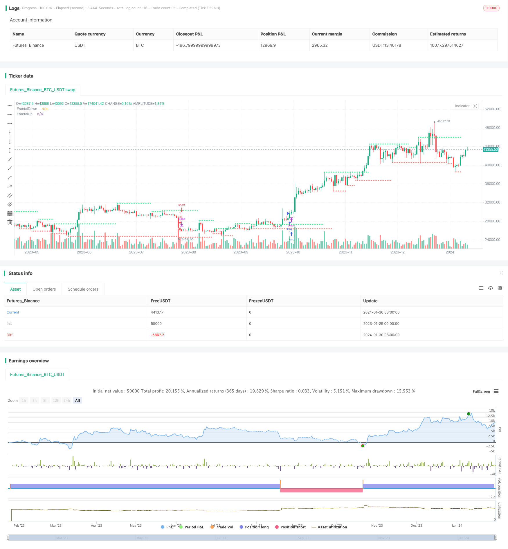
Overview
This strategy uses multi-cycle adaptive moving averages and zigzag risk assessment indicators, combined with phasing points in market operation, to predict trends and output trading signals. The strategy name is "Multi-Cycle Adaptive Trend Forecast Strategy".
Strategy Principle
The core logic of the strategy is divided into two main lines. The first main line utilizes adaptive moving averages nAMA with different parameters to construct a multi-cycle filtering judgment system. The second main line utilizes the zigzag risk assessment system out with different parameters to construct a multi-cycle risk assessment system. Finally, the two main lines are combined. When the short-cycle line exceeds the long-cycle line, a buy signal is generated. When the short-cycle line is below the long-cycle line, a sell signal is generated.
Specifically, the first main line sets adaptive moving averages of 10-cycle and 4, 24 parameters respectively. The second main line sets zigzag risk assessment lines of 7-cycle and 4, 300 parameters respectively. Finally, the 10-cycle line in the first main line is compared with the 31-cycle line in the second main line to form a trading signal. When the 10-cycle line rises above the 31-cycle line, a buy signal is generated. When the 10-cycle line falls below the 31-cycle line, a sell signal is generated.
In addition, the strategy also sets a volume-price confirmation module. Trading signals are only valid when the trading volume is greater than the 6-cycle average trading volume. This can filter out false signals to some extent. Finally, the strategy draws phasing points of different cycle levels as reference signals.
Analysis of Strategy Advantages
The biggest advantage of this strategy is the application of multi-cycle adaptive structures, which can adaptively adjust cycles according to market conditions to dynamically adjust cycles. Whether in trend sections or shock areas, appropriate cycle parameter combinations can be found to improve the strategy's trend-following ability.
In addition, the strategy uses a multi-cycle joint filtering of zigzag risk assessment systems to effectively control trading risks and avoid establishing positions during high-risk phases. At the same time, the strategy also sets volume-price filtering conditions to avoid generating wrong signals when the volume-enabled is insufficient.
Analysis of Strategy Risks
The biggest risk of this strategy is that it requires the same directional judgment of multiple cycle lines, so the ability to capture short-term reversing markets is poor. When short-cycle lines and long-cycle lines change at the same time, unclear signals can be easily generated. Parameter cycles can be shortened for optimization.
In addition, the main cycle phase of the adaptive moving average and zigzag risk assessment system is relatively short compared to the broader market, and there is some lag under the drive of longer levels. The main cycle phase can be appropriately extended to reduce lag.
Strategy Optimization Directions
Shorten the main cycle parameters of the adaptive moving average and zigzag risk assessment line to 5-cycle and 20-cycle to increase capturing of short-term market reversing.
Increase main cycle parameters to 20-cycle and 50-cycle to reduce lag under longer level market drivers.
Optimize trading channel parameters to 0.5 times ATR channel to reduce the possibility of noisy trading.
Add results verification indicators such as MACD to improve signal reliability.
Summary
This strategy comprehensively uses multiple technical indicators such as adaptive moving averages, zigzag risk assessments, and volume-price analysis to construct a multi-cycle adaptive trading decision system. Through optimization and adjustment of parameters, it can be applied to different types of markets, automatically identifying trends and ranges. The strategy logic is clear and valuable to dig into, which is a recommended quant method.
Parameters
| Name | Default | What it controls |
|---|---|---|
| v_input_1 | 10 | Length |
| v_input_2 | 2 | Fastend |
| v_input_3 | 30 | Slowend |
| v_input_4 | 10 | Length2 |
| v_input_5 | 4 | Fastend2 |
| v_input_6 | 24 | Slowend2 |
| v_input_7_hl2 | 0 | price: hl2 | high | low | open | close | hlc3 | hlcc4 | ohlc4 |
| v_input_8 | 7 | len |
| v_input_9 | 4 | FC |
| v_input_10 | 300 | SC |
| v_input_11_hl2 | 0 | price2: hl2 | high | low | open | close | hlc3 | hlcc4 | ohlc4 |
| v_input_12 | 31 | len2 |
| v_input_13 | 40 | FC2 |
| v_input_14 | 300 | SC2 |
| v_input_15 | current | Resolution |
| v_input_16 | 6 | VolumeMA |
Source Pine Script
/*backtest
start: 2023-01-25 00:00:00
end: 2024-01-31 00:00:00
period: 1d
basePeriod: 1h
exchanges: [{"eid":"Futures_Binance","currency":"BTC_USDT"}]
*/

//@version=2
strategy("Best Rabbit Strategy", shorttitle="Rabbit God",overlay=true)
Length = input(10, minval=1)
xPrice = close
xvnoise = abs(xPrice - xPrice[1])
Fastend = input(2)
Slowend = input(30)
nfastend = 2/(Fastend + 1)
nslowend = 2/(Slowend + 1)
nsignal = abs(xPrice - xPrice[Length])
nnoise = sum(xvnoise, Length)
nefratio = iff(nnoise != 0, nsignal / nnoise, 0)
nsmooth = pow(nefratio * (nfastend - nslowend) + nslowend, 2)
nAMA = nz(nAMA[1]) + nsmooth * (xPrice - nz(nAMA[1]))

Length2 = input(10, minval=1)
xPrice2 = close
xvnoise2 = abs(xPrice2 - xPrice2[1])
Fastend2 = input(4)
Slowend2 = input(24)
nfastend2 = 2/(Fastend2 + 1)
nslowend2 = 2/(Slowend2 + 1)
nsignal2 = abs(xPrice2 - xPrice2[Length2])
nnoise2 = sum(xvnoise, Length2)
nefratio2 = iff(nnoise2 != 0, nsignal2 / nnoise2, 0)
nsmooth2 = pow(nefratio2 * (nfastend2 - nslowend2) + nslowend2, 2)
nAMA2 = nz(nAMA2[1]) + nsmooth2 * (xPrice2 - nz(nAMA2[1]))

price = input(hl2)
len = input(defval=7,minval=1)
FC = input(defval=4,minval=1)
SC = input(defval=300,minval=1)
len1 = len/2
w = log(2/(SC+1))
H1 = highest(high,len1)
L1 = lowest(low,len1)
N1 = (H1-L1)/len1
H2 = highest(high,len)[len1]
L2 = lowest(low,len)[len1]
N2 = (H2-L2)/len1
H3 = highest(high,len)
L3 = lowest(low,len)
N3 = (H3-L3)/len
dimen1 = (log(N1+N2)-log(N3))/log(2)
dimen = iff(N1>0 and N2>0 and N3>0,dimen1,nz(dimen1[1]))
alpha1 = exp(w*(dimen-1))
oldalpha = alpha1>1?1:(alpha1<0.01?0.01:alpha1)
oldN = (2-oldalpha)/oldalpha
N = (((SC-FC)*(oldN-1))/(SC-1))+FC
alpha_ = 2/(N+1)
alpha = alpha_<2/(SC+1)?2/(SC+1):(alpha_>1?1:alpha_)
out = (1-alpha)*nz(out[1]) + alpha*price

price2 = input(hl2)
len2 = input(defval=31,minval=1)
FC2 = input(defval=40,minval=1)
SC2 = input(defval=300,minval=1)
len12 = len2/2
w2 = log(2/(SC2+1))
H12 = highest(high,len12)
L12 = lowest(low,len12)
N12 = (H1-L1)/len12
H22 = highest(high,len2)[len12]
L22 = lowest(low,len2)[len12]
N22 = (H22-L22)/len12
H32 = highest(high,len2)
L32 = lowest(low,len2)
N32 = (H32-L32)/len2
dimen12 = (log(N12+N22)-log(N32))/log(2)
dimen2 = iff(N12>0 and N22>0 and N32>0,dimen12,nz(dimen12[1]))
alpha12 = exp(w*(dimen2-1))
oldalpha2 = alpha12>1?1:(alpha12<0.01?0.01:alpha12)
oldN2 = (2-oldalpha2)/oldalpha2
N4 = (((SC2-FC2)*(oldN2-1))/(SC2-1))+FC2
alpha_2 = 2/(N4+1)
alpha2 = alpha_2<2/(SC2+1)?2/(SC2+1):(alpha_2>1?1:alpha_2)
out2 = (1-alpha2)*nz(out2[1]) + alpha2*price2

tf = input(title="Resolution",  defval = "current")
vamp = input(title="VolumeMA",  defval=6)
vam = sma(volume, vamp)

up = high[3]>high[4] and high[4]>high[5] and high[2]<high[3] and high[1]<high[2] and volume[3]>vam[3]
down = low[3]<low[4] and low[4]<low[5] and low[2]>low[3] and low[1]>low[2] and volume[3]>vam[3]
fractalup =  up ? high[3] : fractalup[1]
fractaldown = down ? low[3] : fractaldown[1]

fuptf = request.security(syminfo.tickerid,tf == "current" ? timeframe.period : tf, fractalup)
fdowntf = request.security(syminfo.tickerid,tf == "current" ? timeframe.period : tf, fractaldown)

plot(fuptf, "FractalUp", color=lime, linewidth=1, style=cross, transp=0, offset =-3, join=false)
plot(fdowntf, "FractalDown", color=red, linewidth=1, style=cross, transp=0, offset=-3, join=false)

buyEntry= nAMA[0]>nAMA2[0] and out[0]>out2[0]
sellEntry= nAMA[0]<nAMA2[0] and out[0]<out2[0]

if (buyEntry)
    strategy.entry("Buy", strategy.long, comment="Long Position Entry")


if (sellEntry)
strategy.entry("Sell", strategy.short, comment="Short Position Entry")Published by ChaoZhang on the FMZ strategy square · last modified 2024-02-01. Collected in the Quant Trading Vault. Unvalidated research: re-test with your own data and costs before trusting it.
Build this with AgenKit
A spec is not a trading system. Paste this into your coding agent and AgenKit runs a specialist team — architecture, test-first build, risk gates, review — with paper trading on by default.
/agenkit build a production-grade trading bot with a backtest engine, risk controls and paper trading by default from strategies/Multi-cycle-Adaptive-Trend-Forecast-Strategy.md- npx agenkit install engineering-kit in your project
- Paste the command into your agent and approve each phase
- Get tests, backtest, risk controls and a paper-trading switch
Understand it first
Before you run this, read the lesson behind the idea and how to backtest it honestly. Specs like this one are the survivors of an unknown number of trials; deflate their results accordingly.
Related specs
- ADX MA and EMA Long Only Trend Tracking StrategyPine Script · Trend following · 1d
- ATR and Moving Average Crossover Hybrid StrategyPine Script · Trend following · 1h
- Adaptive FVG Detection and MA Trend Trading Strategy with Dynamic ResistancePine Script · Trend following · 1d
- Adaptive Risk Management Strategy Based on Dynamic ATR and Moving Average CrossoverPine Script · Trend following · 2h
- Adaptive Trading Strategy Based on Stochastic RSI Dual Line CrossoverPine Script · Trend following · 4h
- Adaptive Volatility Based Trend Following Short Strategy with Time Delay and Stop Loss ProtectionPine Script · Trend following · 2m