Parabolic Period and Bollinger Band Combined Moving Stop Loss Strategy

Pine ScriptMean reversion Trend following RSI EMA Bollinger Bands Heikin Ashi Parabolic SAR

Author: ChaoZhang
Complexity: Intermediate · 95 lines
Parameters: 10
Backtest bar: 3h · intraday
Tested on: BTC/USDT · futures

Jump to code View in vault Original on FMZ

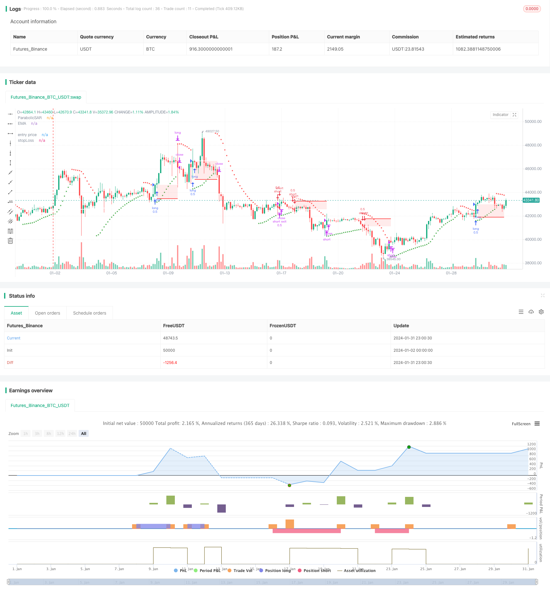
Overview

This article will introduce a quantitative trading strategy that combines the parabolic period indicator and the Bollinger band indicator to set a moving stop loss strategy. By calculating the parabolic period line to judge the market trend direction, and then using the upper and lower rails of the Bollinger bands to dynamically set the stop loss position, the strategy realizes moving stop loss to lock in profits.

Strategy Principle

Firstly, this strategy uses the parabolic indicator to judge the current market trend. When today's closing price crosses above yesterday's parabolic period line, it is considered that the market has reversed to bullish and can go long; when today's closing price crosses below the period line, the market outlook is bearish and can go short.

Secondly, this strategy combines the Bollinger Band indicator to set a dynamic stop loss position. The upper rail of the Bollinger Band can be seen as an overbought zone, and the lower rail is an oversold zone. After going long, if the price falls back below the lower rail of the Bollinger Band, stop loss to close position; after going short, if the price rises above the upper rail again, stop loss to exit. Thus, the upper and lower rails of Bollinger Bands become moving stop loss lines.

Through the above principles, this strategy realizes judging the market direction while setting a dynamic stop loss mechanism to track profits. This allows it to capture some ups and downs in major trends, while also being able to lock in profits through stop losses to avoid risks.

Advantages of the Strategy

Compared with traditional stop loss strategies that only set one fixed stop loss position, this strategy uses the Bollinger band indicator as the stop loss line, so that the stop loss line can move with price fluctuations. This allows it to lock in more profits in relatively large moves. In addition, compared to using the parabolic period line alone, this strategy adds the Bollinger band indicator to determine overbought and oversold areas, which can be more accurate.

Risks and Solutions

The main risk of this strategy is that the trending of the parabolic indicator is not strong. In oscillating markets, prices may cross parabolic period lines several times, causing frequent but small profitable trades for the strategy. At this point, transaction fees and slippage costs may account for a large proportion and reduce the profitability of the strategy.

To cope with the above risks, parameters can be adjusted to increase the degree of change in the parabolic period line to reduce misjudgment probability; or consider combining other indicators to filter entry timing. For example, volatility indicators can be added to determine if the market is trending or oscillating in order to reduce unnecessary trades.

Strategy Optimization

This strategy can be optimized in the following aspects:

Optimize parabolic indicator parameters to adjust indicator change rate to reduce misjudgment probability
Increase other technical indicators filtering, such as adding MACD, KD to determine market type, avoid arbitrage in oscillating market
Optimize Bollinger Band parameters to adjust bandwidth parameters to make Bollinger Bands stick closer to price changes
Increase volume indicators, such as trading volume, positions to assist in judging to avoid false breakouts
Combine fundamentals of stocks to avoid problems with earnings of stocks strategy holding

Summary

This strategy combines judging market trend direction and strength with parabolic indicator, and then uses the upper and lower rails of Bollinger Bands as the moving stop loss position to set a stop loss strategy, achieving a combination of trend tracking and risk control. Compared with traditional fixed stop loss strategies, this strategy can achieve higher returns in larger moves. By optimizing parameters and adding other auxiliary judgment indicators, the stability of the strategy can be further enhanced and unnecessary trades reduced.

Parameters

Name	Default	What it controls
v_input_bool_1	true	(?Backtest Time Period)Filter Date Range of Backtest
v_input_1	timestamp(5 June 2022)	Start Date
v_input_2	timestamp(5 July 2022)	End Date
v_input_int_1	10	(?number of past candles)Swing High
v_input_int_2	10	Swing Low
v_input_int_3	200	(?EMA)Ema Period
v_input_int_4	14	(?RSI)RSI Period
v_input_3	0.02	(?Parabolic SAR)start
v_input_4	0.02	increment
v_input_5	0.2	Max Value

Source Pine Script

/*backtest
start: 2024-01-02 00:00:00
end: 2024-02-01 00:00:00
period: 3h
basePeriod: 15m
exchanges: [{"eid":"Futures_Binance","currency":"BTC_USDT"}]
*/

// This source code is subject to the terms of the Mozilla Public License 2.0 at https://mozilla.org/MPL/2.0/
// © maxencetajet

//@version=5
strategy("HA_RSI", overlay=true, initial_capital=1000, default_qty_type=strategy.fixed, default_qty_value=0.5, slippage=25)

closeHA = request.security(ticker.heikinashi(syminfo.tickerid), timeframe.period, close)

useDateFilter = input.bool(true, title="Filter Date Range of Backtest",
     group="Backtest Time Period")
backtestStartDate = input(timestamp("5 June 2022"), 
     title="Start Date", group="Backtest Time Period",
     tooltip="This start date is in the time zone of the exchange " + 
     "where the chart's instrument trades. It doesn't use the time " + 
     "zone of the chart or of your computer.")
backtestEndDate = input(timestamp("5 July 2022"),
     title="End Date", group="Backtest Time Period",
     tooltip="This end date is in the time zone of the exchange " + 
     "where the chart's instrument trades. It doesn't use the time " + 
     "zone of the chart or of your computer.")

inTradeWindow = true

swingHighV = input.int(10, title="Swing High", group="number of past candles")
swingLowV = input.int(10, title="Swing Low", group="number of past candles")

emaV = input.int(200, title="Ema Period", group="EMA")

rsiV = input.int(14, title="RSI Period", group="RSI")

start = input(0.02, group="Parabolic SAR")
increment = input(0.02, group="Parabolic SAR")
maximum = input(0.2, "Max Value", group="Parabolic SAR")

ema = ta.ema(closeHA, emaV)
rsi = ta.rsi(closeHA, rsiV)
SAR = ta.sar(start, increment, maximum)

myColor = SAR < low?color.green:color.red

longcondition = closeHA > ema and rsi > 50 and closeHA[1] > SAR and closeHA[1] < SAR[1] 
shortcondition = closeHA < ema and rsi < 50 and closeHA[1] < SAR and closeHA[1] > SAR[1]

float risk_long = na
float risk_short = na
float stopLoss = na
float entry_price = na
float takeProfit = na

risk_long := risk_long[1]
risk_short := risk_short[1]

swingHigh = ta.highest(closeHA, swingHighV)
swingLow = ta.lowest(closeHA, swingLowV)

if strategy.position_size == 0 and longcondition and inTradeWindow
    risk_long := (close - swingLow) / close
    strategy.entry("long", strategy.long, comment="Buy")
    
if strategy.position_size == 0 and shortcondition and inTradeWindow
    risk_short := (swingHigh - close) / close       
    strategy.entry("short", strategy.short, comment="Sell")
    
if strategy.position_size > 0

    stopLoss := strategy.position_avg_price * (1 - risk_long)
    entry_price := strategy.position_avg_price
    strategy.exit("long exit", "long", stop = stopLoss)
    
if strategy.position_size < 0 

    stopLoss := strategy.position_avg_price * (1 + risk_short)
    entry_price := strategy.position_avg_price
    strategy.exit("short exit", "short", stop = stopLoss)

if closeHA[1] < SAR and close > strategy.position_avg_price
    strategy.close("long", comment="Exit Long")
    
if closeHA[1] > SAR and close < strategy.position_avg_price
    strategy.close("short", comment="Exit Short")

p_ep = plot(entry_price, color=color.new(color.white, 0), linewidth=2, style=plot.style_linebr, title='entry price')
p_sl = plot(stopLoss, color=color.new(color.red, 0), linewidth=2, style=plot.style_linebr, title='stopLoss')
fill(p_sl, p_ep, color.new(color.red, transp=85))

plot(SAR, "ParabolicSAR", style=plot.style_circles, color=myColor, linewidth=1)
plot(ema, color=color.white, linewidth=2, title="EMA")

Published by ChaoZhang on the FMZ strategy square · last modified 2024-02-02. Collected in the Quant Trading Vault. Unvalidated research: re-test with your own data and costs before trusting it.

Build this with AgenKit

A spec is not a trading system. Paste this into your coding agent and AgenKit runs a specialist team — architecture, test-first build, risk gates, review — with paper trading on by default.

in Claude Code, Cursor, Codex & 4 more

/agenkit build a production-grade trading bot with a backtest engine, risk controls and paper trading by default from strategies/Parabolic-Period-and-Bollinger-Band-Combined-Moving-Stop-Loss-Strategy.md

npx agenkit install engineering-kit in your project
Paste the command into your agent and approve each phase
Get tests, backtest, risk controls and a paper-trading switch

Get AgenKit How /agenkit works

Understand it first

Before you run this, read the lesson behind the idea and how to backtest it honestly. Specs like this one are the survivors of an unknown number of trials; deflate their results accordingly.