Pivot Reversal Based Quantitative Trading Strategy

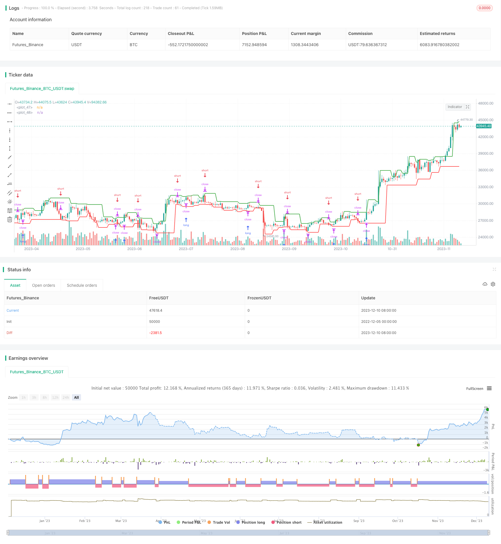
This is a quantitative trading strategy that utilizes pivot points as entry signals. It calculates rising pivot points and falling pivot points. Once the price breaks through these pivot points, it will initiate long…

Pine ScriptMean reversion Breakout Momentum Pivots / S&R

Author: ChaoZhang
Complexity: Advanced · 339 lines
Parameters: 10
Backtest bar: 1d · swing
Tested on: BTC/USDT · futures

Jump to code View in vault Original on FMZ

Overview

Strategy Principle

This strategy is mainly based on the pivot reversal theory. It first calculates the pivot points based on the left N bars and right M bars. Then it monitors in real time whether the price breaks through these pivot points.

When the price breaks through the rising pivot point, it means the upward momentum is no longer enough to continue pushing up the price. At this time, going short can yield good returns. When the price breaks through the falling pivot point, it means that the downward momentum has been exhausted. At this time, going long can obtain good returns.

Specifically, this strategy calculates the rising pivot points and falling pivot points through the ta.pivothigh and ta.pivotlow functions. Then it compares whether the current highest price breaks through the rising pivot point and whether the lowest price breaks through the falling pivot point. If there is a breakthrough, the corresponding long or short strategy will be initiated.

In addition, this strategy also uses stop loss to control risks. Specifically, when the price breaks through the pivot point, it immediately places an order while setting the stop loss at the other side of the pivot point. This can minimize the loss caused by a failed signal.

Advantage Analysis

This pivot reversal based strategy has the following advantages:

The pivot reversal signal is quite reliable with a high winning rate
The risk is well controlled with reasonable stop loss setting
It's easy to implement with concise code
It is applicable to different products with good flexibility

Risk Analysis

This strategy also has some risks to note:

The pivot points may fail, resulting in incorrect signals
There could be pullback after breaking the pivot point, causing stop loss triggering
The trading frequency may be high, incurring implicit trading cost
The performance relies on product selection and parameter tuning

To reduce risks, the following aspects can be considered:

Optimize the number of left and right bars to ensure reliable pivot point calculation
Loose the stop loss to some extent to avoid over-tightness
Set minimum profit target to reduce frequent round-trip trading
Test on different products and parameters to find the optimal configuration

Optimization Directions

There is room for further optimization of this strategy:

Incorporate other indicators to judge the reliability of pivot breakthroughs
Add machine learning models to determine price trends
Use high-frequency data to improve signal sensitivity
Introduce position sizing module to dynamically adjust positions
Connect detailed account module to calculate real trading cost

These optimizations could improve the win rate, profitability, and stability of the strategy.

Conclusion

In summary, this is a quantitative trading strategy based on the pivot reversal theory. It uses price breakthrough pivot points as trading signals while adopting stop loss to control risks. This strategy is easy to implement and widely applicable, making it a practical quantitative trading strategy. But it also bears some risks and needs further testing and optimization to find the optimal configuration in real trading.

Parameters

Name	Default	What it controls
v_input_1	2	(?Pivot Points)leftBars
v_input_2	true	rightBars
v_input_3	true	(?Weekly Table)Return Precision
v_input_4	timestamp(01 Jan 3000 00:00 +0000)	(?Weekhly Table)From Date
v_input_color_1	green	(?Weeky Table)Gradient Colors
v_input_color_2	red	loss_color
v_input_bool_1	true	(?Benchmark)Use current Symbol for Benchmark
v_input_5	BTC_USDT:swap	Benchmark
v_input_bool_2	false	Display Benchmark?
v_input_bool_3	false	Display Alpha?

Source Pine Script

/*backtest
start: 2022-12-05 00:00:00
end: 2023-12-11 00:00:00
period: 1d
basePeriod: 1h
exchanges: [{"eid":"Futures_Binance","currency":"BTC_USDT"}]
*/

//@version=5
strategy('Weekly Returns with Benchmark', overlay=true, 
     default_qty_type=strategy.percent_of_equity, default_qty_value=25, 
     commission_type=strategy.commission.percent, commission_value=0.1)

////////////
// Inputs //

// Pivot points inputs
leftBars   = input(2, group = "Pivot Points")
rightBars  = input(1, group = "Pivot Points")

// Styling inputs
prec       = input(1, title='Return Precision',                            group = "Weekly Table")
from_date  = input(timestamp("01 Jan 3000 00:00 +0000"), "From Date", group = "Weekhly Table")
prof_color = input.color(color.green, title = "Gradient Colors", group = "Weeky Table", inline = "colors")
loss_color = input.color(color.red,   title = "",                group = "Weeky Table", inline = "colors")

// Benchmark inputs
use_cur    = input.bool(true,        title = "Use current Symbol for Benchmark", group = "Benchmark")
symb_bench = input('BTC_USDT:swap', title = "Benchmark",                        group = "Benchmark")
disp_bench = input.bool(false,       title = "Display Benchmark?",               group = "Benchmark")
disp_alpha = input.bool(false,       title = "Display Alpha?",                   group = "Benchmark")

// Pivot Points Strategy
swh = ta.pivothigh(leftBars, rightBars)
swl = ta.pivotlow (leftBars, rightBars)

hprice = 0.0
hprice := not na(swh) ? swh : hprice[1]

lprice = 0.0
lprice := not na(swl) ? swl : lprice[1]

le = false
le := not na(swh) ? true : le[1] and high > hprice ? false : le[1]

se = false
se := not na(swl) ? true : se[1] and low < lprice ? false : se[1]

if le
    strategy.entry('PivRevLE', strategy.long, comment='PivRevLE', stop=hprice + syminfo.mintick)

if se
    strategy.entry('PivRevSE', strategy.short, comment='PivRevSE', stop=lprice - syminfo.mintick)

plot(hprice, color=color.new(color.green, 0), linewidth=2)
plot(lprice, color=color.new(color.red, 0), linewidth=2)


///////////////////
// WEEKLY TABLE //

new_week = weekofyear(time[1]) != weekofyear(time)
new_year = year(time) != year(time[1])

eq       = strategy.equity
bench_eq = close

// benchmark eq
bench_eq_htf = request.security(symb_bench, timeframe.period, close)

if (not use_cur)
    bench_eq := bench_eq_htf

bar_pnl   = eq / eq[1] - 1
bench_pnl = bench_eq / bench_eq[1] - 1



// Current Weekly P&L
cur_week_pnl  = 0.0
cur_week_pnl := bar_index == 0 ? 0 : 
                 time >= from_date and (time[1] < from_date or new_week) ? bar_pnl : 
                 (1 + cur_week_pnl[1]) * (1 + bar_pnl) - 1

// Current Yearly P&L
cur_year_pnl  = 0.0
cur_year_pnl := bar_index == 0 ? 0 : 
                 time >= from_date and (time[1] < from_date or new_year) ? bar_pnl : 
                 (1 + cur_year_pnl[1]) * (1 + bar_pnl) - 1


// Current Weekly P&L - Bench
bench_cur_week_pnl  = 0.0
bench_cur_week_pnl := bar_index == 0 or (time[1] < from_date and time >= from_date) ? 0 : 
                       time >= from_date and new_week ? bench_pnl : 
                       (1 + bench_cur_week_pnl[1]) * (1 + bench_pnl) - 1 

// Current Yearly P&L - Bench
bench_cur_year_pnl  = 0.0
bench_cur_year_pnl := bar_index == 0 ? 0 : 
                       time >= from_date and (time[1] < from_date  or new_year) ? bench_pnl : 
                       (1 + bench_cur_year_pnl[1]) * (1 + bench_pnl) - 1




var week_time = array.new_int(0)
var year_time = array.new_int(0)

var week_pnl = array.new_float(0)
var year_pnl = array.new_float(0)

var bench_week_pnl = array.new_float(0)
var bench_year_pnl = array.new_float(0)


// Filling weekly / yearly pnl arrays
if array.size(week_time) > 0
    if weekofyear(time) == weekofyear(array.get(week_time, array.size(week_time) - 1))
        array.pop(week_pnl)
        array.pop(bench_week_pnl)
        array.pop(week_time)


if array.size(year_time) > 0
    if year(time) == year(array.get(year_time, array.size(year_time) - 1))
        array.pop(year_pnl)
        array.pop(bench_year_pnl)
        array.pop(year_time)


if (time >= from_date)
    array.push(week_time, time)
    array.push(year_time, time)
    
    array.push(week_pnl, cur_week_pnl)
    array.push(year_pnl, cur_year_pnl)
    
    array.push(bench_year_pnl, bench_cur_year_pnl)
    array.push(bench_week_pnl, bench_cur_week_pnl)


// Weekly P&L Table  

table_size = size.tiny
var weekly_table = table(na)

if array.size(year_pnl) > 0 and barstate.islastconfirmedhistory

    weekly_table := table.new(position.bottom_right, 
                 columns=56, rows=array.size(year_pnl) * 3 + 5, border_width=1)

// Fill weekly performance
    table.cell(weekly_table, 0, 0,  'Perf', 
                 bgcolor = #999999, text_size= table_size)


    for numW = 1 to 53 by 1
        table.cell(weekly_table, numW, 0,  str.tostring(numW), 
                 bgcolor= #999999, text_size= table_size)


    table.cell(weekly_table, 54, 0, ' ',    
                 bgcolor = #999999, text_size= table_size)
    table.cell(weekly_table, 55, 0, 'Year', 
                 bgcolor = #999999, text_size= table_size)

    max_abs_y = math.max(math.abs(array.max(year_pnl)), math.abs(array.min(year_pnl)))
    max_abs_m = math.max(math.abs(array.max(week_pnl)), math.abs(array.min(week_pnl)))

    
    for yi = 0 to array.size(year_pnl) - 1 by 1
        table.cell(weekly_table, 0,  yi + 1,
                 str.tostring(year(array.get(year_time, yi))), 
                 bgcolor=#cccccc, text_size=table_size)
                 
        table.cell(weekly_table, 53, yi + 1, ' ',   
                 bgcolor=#999999, text_size=table_size)
                 
        table.cell(weekly_table, 54, yi + 1, ' ',   
                 bgcolor=#999999, text_size=table_size)

        y_color = color.from_gradient(array.get(year_pnl, yi), -max_abs_y, max_abs_y, loss_color, prof_color) 

        table.cell(weekly_table, 55, yi + 1, 
                 str.tostring(math.round(array.get(year_pnl, yi) * 100, prec)), 
                 bgcolor=y_color, text_size=table_size)
    
    int iw_row= na
    int iw_col= na

    for wi = 0 to array.size(week_time) - 2 by 1
        w_row   = year(array.get(week_time, wi)) - year(array.get(year_time, 0)) + 1
        w_col   = weekofyear(array.get(week_time, wi))

        w_color = color.from_gradient(array.get(week_pnl, wi), -max_abs_m, max_abs_m, loss_color, prof_color)
        
        if iw_row + 1 == w_row and iw_col + 1 == w_col
            table.cell(weekly_table, w_col, w_row-1,
                 str.tostring(math.round(array.get(week_pnl, wi) * 100, prec)), 
                 bgcolor=w_color, text_size=table_size)
        else
            table.cell(weekly_table, w_col, w_row,
                 str.tostring(math.round(array.get(week_pnl, wi) * 100, prec)), 
                 bgcolor=w_color, text_size=table_size)
        
        
        iw_row:= w_row
        iw_col:= w_col


    // Fill benchmark performance
    next_row =  array.size(year_pnl) + 1  

    if (disp_bench)
    
        table.cell(weekly_table, 0,  next_row, 'Bench', 
                 bgcolor=#999999, text_size=table_size)
        
        for numW = 1 to 53 by 1
            table.cell(weekly_table, numW, next_row,  str.tostring(numW), 
                 bgcolor= #999999, text_size= table_size)

        table.cell(weekly_table, 54, next_row, ' '   ,   
                 bgcolor = #999999, text_size=table_size)
        table.cell(weekly_table, 55, next_row, 'Year',   
                 bgcolor = #999999, text_size=table_size)
    
        max_bench_abs_y = math.max(math.abs(array.max(bench_year_pnl)), math.abs(array.min(bench_year_pnl)))
        max_bench_abs_w = math.max(math.abs(array.max(bench_week_pnl)), math.abs(array.min(bench_week_pnl)))
    
        for yi = 0 to array.size(year_time) - 1 by 1
            table.cell(weekly_table, 0,  yi + 1 + next_row + 1, 
                 str.tostring(year(array.get(year_time, yi))), 
                 bgcolor=#cccccc, text_size=table_size)

            table.cell(weekly_table, 53, yi + 1 + next_row + 1, ' ',   
                 bgcolor=#999999, text_size=table_size)
            
            table.cell(weekly_table, 54, yi + 1 + next_row + 1, ' ', 
                 bgcolor=#999999, text_size=table_size)
                 
            y_color = color.from_gradient(array.get(bench_year_pnl, yi), -max_bench_abs_y, max_bench_abs_y, loss_color, prof_color)
            table.cell(weekly_table, 55, yi + 1 + next_row + 1, 
                 str.tostring(math.round(array.get(bench_year_pnl, yi) * 100, prec)), 
                 bgcolor=y_color, text_size=table_size)
     
    
        int iw_row1= na
        int iw_col1= na

        for wi = 0 to array.size(week_time) - 1 by 1
            w_row   = year(array.get(week_time, wi)) - year(array.get(year_time, 0)) + 1
            w_col   = weekofyear(array.get(week_time, wi))
        
            w_color = color.from_gradient(array.get(bench_week_pnl, wi), -max_bench_abs_w, max_bench_abs_w, loss_color, prof_color)
    
            if iw_row1 + 1 == w_row and iw_col1 + 1 == w_col
                table.cell(weekly_table, w_col, w_row  + next_row    , 
                 str.tostring(math.round(array.get(bench_week_pnl, wi) * 100, prec)),
                 bgcolor=w_color, text_size=table_size)
            else
                table.cell(weekly_table, w_col, w_row  + next_row + 1, 
                 str.tostring(math.round(array.get(bench_week_pnl, wi) * 100, prec)), 
                 bgcolor=w_color, text_size=table_size)
                
            iw_row1:= w_row
            iw_col1:= w_col
    
    
// Fill Alpha
    if (disp_alpha)
    
        // columns
        next_row :=  array.size(year_pnl) * 2 + 3   
        table.cell(weekly_table, 0,  next_row, 'Alpha', 
                 bgcolor=#999999, text_size= table_size)


        for numW = 1 to 53 by 1
            table.cell(weekly_table, numW, next_row,  str.tostring(numW), 
                 bgcolor= #999999, text_size= table_size)


        table.cell(weekly_table, 54, next_row, ' '   ,  
                 bgcolor=#999999, text_size= table_size)
        table.cell(weekly_table, 55, next_row, 'Year',  
                 bgcolor=#999999, text_size= table_size)
        
        
        
        max_alpha_abs_y = 0.0
        for yi = 0 to array.size(year_time) - 1 by 1
            if (math.abs(array.get(year_pnl, yi)  - array.get(bench_year_pnl, yi)) > max_alpha_abs_y)
                max_alpha_abs_y := math.abs(array.get(year_pnl, yi)  - array.get(bench_year_pnl, yi))
    
        max_alpha_abs_w = 0.0
        for wi = 0 to array.size(week_pnl) - 1 by 1
            if (math.abs(array.get(week_pnl, wi) - array.get(bench_week_pnl, wi)) > max_alpha_abs_w)
                max_alpha_abs_w := math.abs(array.get(week_pnl, wi) - array.get(bench_week_pnl, wi))
    
    
        for yi = 0 to array.size(year_time) - 1 by 1
            table.cell(weekly_table, 0,  yi + 1 + next_row + 1, 
                 str.tostring(year(array.get(year_time, yi))), 
                 bgcolor=#cccccc, text_size= table_size)
                 
            table.cell(weekly_table, 53, yi + 1 + next_row + 1, ' ',   
                 bgcolor=#999999, text_size= table_size)
                 
            table.cell(weekly_table, 54, yi + 1 + next_row + 1, ' ',   
                 bgcolor=#999999, text_size= table_size)

            y_color = color.from_gradient(array.get(year_pnl, yi)  - array.get(bench_year_pnl, yi), -max_alpha_abs_y, max_alpha_abs_y, loss_color, prof_color)
            table.cell(weekly_table, 55, yi + 1 + next_row + 1,
                 str.tostring(math.round((array.get(year_pnl, yi)  - array.get(bench_year_pnl, yi)) * 100, prec)), 
                 bgcolor=y_color, text_size= table_size)
     
     
        int iw_row2= na
        int iw_col2= na
        
        for wi = 0 to array.size(week_time) - 1 by 1
            w_row   = year(array.get(week_time, wi)) - year(array.get(year_time, 0)) + 1
            w_col   = weekofyear(array.get(week_time, wi))
            w_color = color.from_gradient(array.get(week_pnl, wi) - array.get(bench_week_pnl, wi), -max_alpha_abs_w, max_alpha_abs_w, loss_color, prof_color)
    
            if iw_row2 + 1 == w_row and iw_col2 + 1 == w_col
                table.cell(weekly_table, w_col, w_row  + next_row , 
                     str.tostring(math.round((array.get(week_pnl, wi) - array.get(bench_week_pnl, wi)) * 100, prec)), 
                     bgcolor=w_color, text_size= table_size)
            else
                table.cell(weekly_table, w_col, w_row  + next_row + 1 , 
                     str.tostring(math.round((array.get(week_pnl, wi) - array.get(bench_week_pnl, wi)) * 100, prec)), 
                     bgcolor=w_color, text_size= table_size)
        
            iw_row2:= w_row
            iw_col2:= w_col

Published by ChaoZhang on the FMZ strategy square · last modified 2023-12-12. Collected in the Quant Trading Vault. Unvalidated research: re-test with your own data and costs before trusting it.

Build this with AgenKit

A spec is not a trading system. Paste this into your coding agent and AgenKit runs a specialist team — architecture, test-first build, risk gates, review — with paper trading on by default.

in Claude Code, Cursor, Codex & 4 more

/agenkit build a production-grade trading bot with a backtest engine, risk controls and paper trading by default from strategies/Pivot-Reversal-Based-Quantitative-Trading-Strategy.md

npx agenkit install engineering-kit in your project
Paste the command into your agent and approve each phase
Get tests, backtest, risk controls and a paper-trading switch

Get AgenKit How /agenkit works

Understand it first

Before you run this, read the lesson behind the idea and how to backtest it honestly. Specs like this one are the survivors of an unknown number of trials; deflate their results accordingly.