Strategy vault / Trend following
Trend Following Strategy Based on Time Series Decomposition and Volume Weighted Bollinger Bands
This strategy integrates time series decomposition, volume weighted average price, Bollinger Bands and delta(OBV-PVT) 4 technical indicators to make multidimensional judgments on price trends, overbought and oversold…
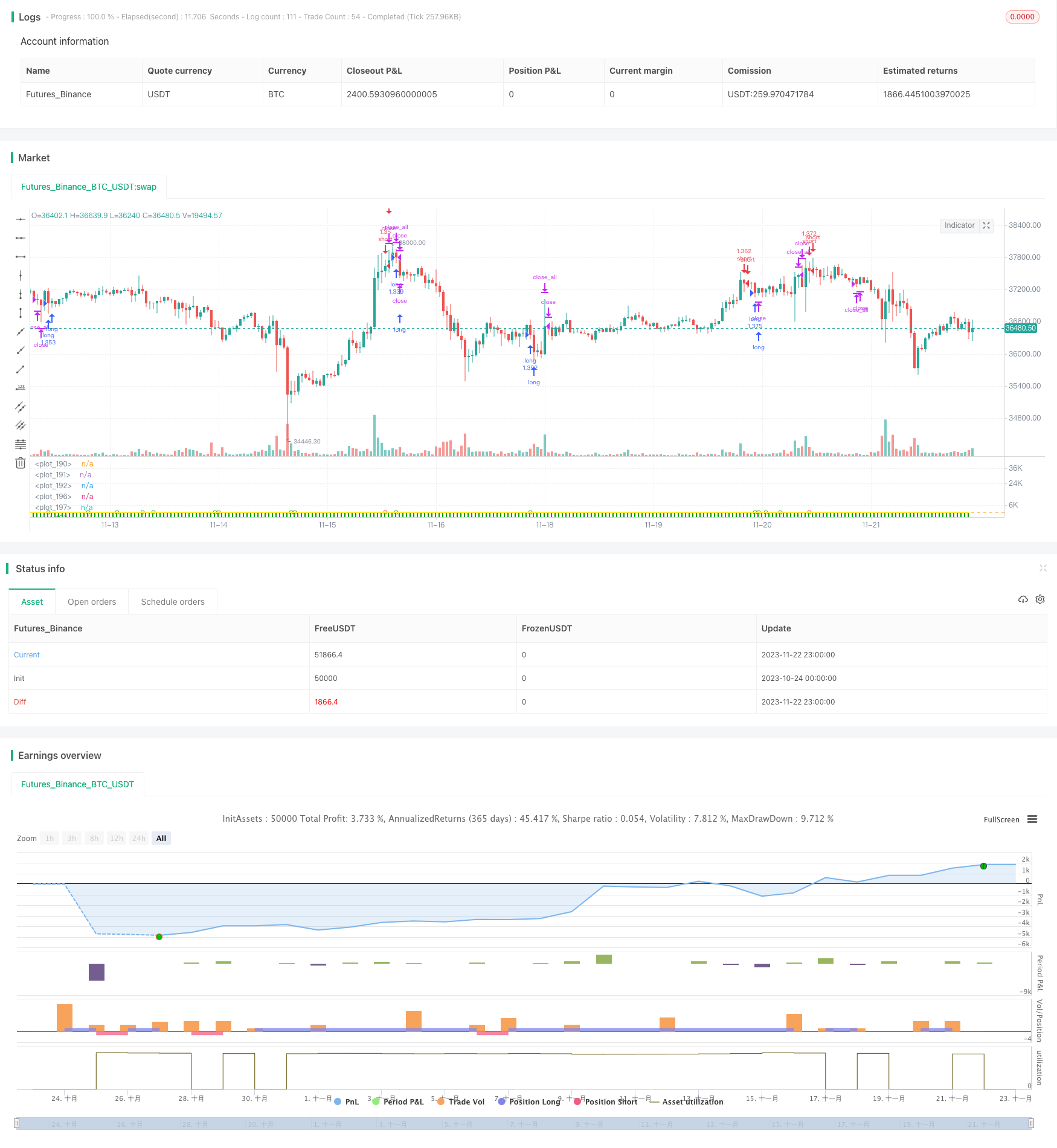
Overview
This strategy integrates time series decomposition, volume weighted average price, Bollinger Bands and delta(OBV-PVT) 4 technical indicators to make multidimensional judgments on price trends, overbought and oversold conditions.
Principles
- Use time series decomposition to remove noise and periodicity in prices for more accurate trend judgment;
- Calculate volume weighted new price based on the trend line;
- Calculate the Bollinger Bands Percentage Width (BB%B) of closing price to determine overbought and oversold conditions;
- Calculate the BB%B of Delta(OBV-PVT) as a measure of price-volume divergence;
- Generate trading signals based on price-volume indicators crosses and Bollinger Bands overshoots and undershoots.
Advantages
- Combines price, volume and statistical features for robust judgments;
- BB%B combined with Delta(OBV-PVT) better identifies short-term overbought/oversold conditions;
- Price-volume crossover signals filter out some false signals.
Risks
- Too complex parameter tuning;
- Short-term choppiness may increase losses;
- Price-volume divergences do not completely filter false signals.
Parameters like moving averages, Bollinger Bands widths and risk-reward ratios can be optimized to reduce trading frequency while improving risk-adjusted returns per trade.
Conclusion
Integrating tools like time series decomposition, Bollinger Bands, OBV indicators, this strategy combines price-volume relationships, statistical properties and trend analysis to identify short-term reversals and catch major trends. There are also certain risks that need to be addressed through parameter tuning for optimal performance.
Parameters
| Name | Default | What it controls |
|---|---|---|
| v_input_1 | true | Start Date |
| v_input_2 | true | Start Month |
| v_input_3 | 2010 | Start Year |
| v_input_4 | 31 | End Date |
| v_input_5 | 12 | End Month |
| v_input_6 | 2021 | End Year |
| v_input_7 | 2 | Stop Loss % |
| v_input_8 | 4 | Take Profit % |
| v_input_9 | 20 | length |
| v_input_10 | 2 | StdDev |
| v_input_11 | 1000 | Smoothing Factor (Lambda) |
| v_input_12 | 100 | Filter Length |
| v_input_13 | 1 | TimeFrame |
| v_input_14 | false | Show barcolors |
| v_input_15 | false | Show previous VWAP close |
| v_input_16 | 20 | l1 |
| v_input_17 | 2 | StdDev |
| v_input_18 | 0.3 | xx |
| v_input_19 | 0.7 | yy |
| v_input_20 | -1 | zz |
| v_input_21 | 16 | Period |
Source Pine Script
/*backtest
start: 2023-10-24 00:00:00
end: 2023-11-23 00:00:00
period: 1h
basePeriod: 15m
exchanges: [{"eid":"Futures_Binance","currency":"BTC_USDT"}]
*/

// This source code is subject to the terms of the Mozilla Public License 2.0 at https://mozilla.org/MPL/2.0/
//// This source code is subject to the terms of the Mozilla Public License 2.0 at https://mozilla.org/MPL/2.0/
// © oakwhiz and tathal

//@version=4
strategy("BBPBΔ(OBV-PVT)BB", default_qty_type=strategy.percent_of_equity, default_qty_value=100)

startDate = input(title="Start Date", type=input.integer,
     defval=1, minval=1, maxval=31)
startMonth = input(title="Start Month", type=input.integer,
     defval=1, minval=1, maxval=12)
startYear = input(title="Start Year", type=input.integer,
     defval=2010, minval=1800, maxval=2100)

endDate = input(title="End Date", type=input.integer,
     defval=31, minval=1, maxval=31)
endMonth = input(title="End Month", type=input.integer,
     defval=12, minval=1, maxval=12)
endYear = input(title="End Year", type=input.integer,
     defval=2021, minval=1800, maxval=2100)

// Normalize Function
normalize(_src, _min, _max) =>
    // Normalizes series with unknown min/max using historical min/max.
    // _src      : series to rescale.
    // _min, _min: min/max values of rescaled series.
    var _historicMin =  10e10
    var _historicMax = -10e10
    _historicMin := min(nz(_src, _historicMin), _historicMin)
    _historicMax := max(nz(_src, _historicMax), _historicMax)
    _min + (_max - _min) * (_src - _historicMin) / max(_historicMax - _historicMin, 10e-10)


// STEP 2:
// Look if the close time of the current bar
// falls inside the date range
inDateRange = true


// Stop loss & Take Profit Section
sl_inp = input(2.0, title='Stop Loss %')/100
tp_inp = input(4.0, title='Take Profit %')/100

stop_level = strategy.position_avg_price * (1 - sl_inp)
take_level = strategy.position_avg_price * (1 + tp_inp)

icreturn = false
innercandle = if (high < high[1]) and (low > low[1])
    icreturn := true

src = close

float change_src = change(src)
float i_obv = cum(change_src > 0 ? volume : change_src < 0 ? -volume : 0*volume)
float i_pvt = pvt

float result = change(i_obv - i_pvt)

float nresult = ema(normalize(result, -1, 1), 20)


length = input(20, minval=1)
mult = input(2.0, minval=0.001, maxval=50, title="StdDev")
basis = ema(nresult, length)
dev = mult * stdev(nresult, length)
upper = basis + dev
lower = basis - dev
bbr = (nresult - lower)/(upper - lower)


////////////////INPUTS///////////////////
lambda = input(defval = 1000, type = input.float, title = "Smoothing Factor (Lambda)", minval = 1)
leng = input(defval = 100, type = input.integer, title = "Filter Length", minval = 1)
srcc = close

///////////Construct Arrays///////////////
a = array.new_float(leng, 0.0)
b = array.new_float(leng, 0.0)
c = array.new_float(leng, 0.0)
d = array.new_float(leng, 0.0)
e = array.new_float(leng, 0.0)
f = array.new_float(leng, 0.0)

/////////Initialize the Values///////////
//for more details visit:
//          https://asmquantmacro.com/2015/06/25/hodrick-prescott-filter-in-excel/

ll1 = leng-1
ll2 = leng-2

for i = 0 to ll1
    array.set(a,i, lambda*(-4))
    array.set(b,i, src[i])
    array.set(c,i, lambda*(-4))
    array.set(d,i, lambda*6 + 1)
    array.set(e,i, lambda)
    array.set(f,i, lambda)

array.set(d, 0,  lambda + 1.0)
array.set(d, ll1, lambda + 1.0)
array.set(d, 1,  lambda * 5.0 + 1.0)
array.set(d, ll2, lambda * 5.0 + 1.0)

array.set(c, 0 , lambda * (-2.0))
array.set(c, ll2, lambda * (-2.0))

array.set(a, 0 , lambda * (-2.0))
array.set(a, ll2, lambda * (-2.0))

//////////////Solve the optimization issue/////////////////////
float r = array.get(a, 0)
float s = array.get(a, 1)
float t = array.get(e, 0)
float xmult = 0.0

for i = 1 to ll2
    xmult := r / array.get(d, i-1)
    array.set(d, i, array.get(d, i) - xmult * array.get(c, i-1))
    array.set(c, i, array.get(c, i) - xmult * array.get(f, i-1))
    array.set(b, i, array.get(b, i) - xmult * array.get(b, i-1))

    xmult := t / array.get(d, i-1)
    r     := s - xmult*array.get(c, i-1)
    array.set(d, i+1, array.get(d, i+1) - xmult * array.get(f, i-1))
    array.set(b, i+1, array.get(b, i+1) - xmult * array.get(b, i-1))

    s     := array.get(a, i+1)
    t     := array.get(e, i)

xmult := r / array.get(d, ll2)
array.set(d, ll1, array.get(d, ll1) - xmult * array.get(c, ll2))

x = array.new_float(leng, 0)
array.set(x, ll1, (array.get(b, ll1) - xmult * array.get(b, ll2)) / array.get(d, ll1))
array.set(x, ll2, (array.get(b, ll2) - array.get(c, ll2) * array.get(x, ll1)) / array.get(d, ll2))

for j = 0 to leng-3
    i = leng-3 - j
    array.set(x, i, (array.get(b,i) - array.get(f,i)*array.get(x,i+2) - array.get(c,i)*array.get(x,i+1)) / array.get(d, i))


//////////////Construct the output///////////////////
o5 = array.get(x,0)

////////////////////Plottingd///////////////////////


TimeFrame = input('1', type=input.resolution)
start = security(syminfo.tickerid, TimeFrame, time)

//------------------------------------------------
newSession = iff(change(start), 1, 0)
//------------------------------------------------
vwapsum = 0.0
vwapsum := iff(newSession, o5*volume, vwapsum[1]+o5*volume)
volumesum = 0.0
volumesum := iff(newSession, volume, volumesum[1]+volume)
v2sum = 0.0
v2sum := iff(newSession, volume*o5*o5, v2sum[1]+volume*o5*o5)
myvwap = vwapsum/volumesum
dev2 = sqrt(max(v2sum/volumesum - myvwap*myvwap, 0))
Coloring=close>myvwap?color.green:color.red
av=myvwap
showBcol = input(false, type=input.bool, title="Show barcolors")
showPrevVWAP = input(false, type=input.bool, title="Show previous VWAP close")
prevwap = 0.0
prevwap := iff(newSession, myvwap[1], prevwap[1])
nprevwap= normalize(prevwap, 0, 1)

l1= input(20, minval=1)
src2 = close
mult1 = input(2.0, minval=0.001, maxval=50, title="StdDev")
basis1 = sma(src2, l1)
dev1 = mult1 * stdev(src2, l1)
upper1 = basis1 + dev1
lower1 = basis1 - dev1
bbr1 = (src - lower1)/(upper1 - lower1)

az = plot(bbr, "Δ(OBV-PVT)", color.rgb(0,153,0,0), style=plot.style_columns)
bz = plot(bbr1, "BB%B", color.rgb(0,125,125,50), style=plot.style_columns)
fill(az, bz, color=color.white)


deltabbr = bbr1 - bbr
oneline = hline(1)
twoline = hline(1.2)
zline = hline(0)
xx = input(.3)
yy = input(.7)
zz = input(-1)
xxx = hline(xx)
yyy = hline(yy)
zzz = hline(zz)
fill(oneline, twoline, color=color.red, title="Sell Zone")
fill(yyy, oneline, color=color.orange, title="Slightly Overbought")
fill(yyy, zline, color=color.white, title="DO NOTHING ZONE")
fill(zzz, zline, color=color.green, title="GO LONG ZONE")

l20 = crossover(deltabbr, 0)
l30 = crossunder(deltabbr, 0)
l40 = crossover(o5, 0)
l50 = crossunder(o5, 0)


z1 = bbr1 >= 1
z2 = bbr1 < 1 and bbr1 >= .7
z3 = bbr1 < .7 and bbr1 >= .3
z4 = bbr1 < .3 and bbr1 >= 0
z5 = bbr1 < 0
a1 = bbr >= 1
a2 = bbr < 1 and bbr >= .7

a4 = bbr < .3 and bbr >= 0
a5 = bbr < 0
b4 = deltabbr < .3 and deltabbr >= 0
b5 = deltabbr < 0
c4 = o5 < .3 and o5 >= 0
c5 = o5 < 0
b1 = deltabbr >= 1
b2 = deltabbr < 1 and o5 >= .7
c1 = o5 >= 1
c2 = o5 < 1 and o5 >= .7

///

n = input(16,"Period")
H = highest(hl2,n)
L = lowest(hl2,n)
hi = H[1]
lo = L[1]
up = high>hi
dn = low<lo
lowerbbh = lowest(10)[1]
bbh = (low == open ?  open < lowerbbh ? open < close ? close > ((high[1] - low[1]) / 2) + low[1] :na  : na : na)


plot(normalize(av,-1,1), linewidth=2, title="Trendline", color=color.yellow)


long5 = close < av and av[0] > av[1]
sell5 = close > av

cancel = false
if open >= high[1]
    cancel = true


long = (long5 or z5 or a5) and (icreturn or bbh or up)
sell = ((z1 or a1) or (l40 and l20)) and (icreturn or dn) and (c1 or b1)
short = ((z1 or z2 or a1 or sell5) and (l40 or l20)) and icreturn
buy= (z5 or z4 or a5 or long5) and (icreturn or dn)


plotshape(long and not sell ? -0.5 : na, title="Long", location=location.absolute, style=shape.circle, size=size.tiny, color=color.green, transp=0)
plotshape(short and not sell? 1 : na, title="Short", location=location.absolute, style=shape.circle, size=size.tiny, color=color.red, transp=0)


if (inDateRange)
    strategy.entry("long", true, when = long )

if (inDateRange) and (strategy.position_size > 0)
    strategy.close_all(when = sell or cancel)


if (inDateRange)
    strategy.entry("short", false, when = short )

if (inDateRange) and (strategy.position_size < 0)
strategy.close_all(when = buy)Published by ChaoZhang on the FMZ strategy square · last modified 2023-11-24. Collected in the Quant Trading Vault. Unvalidated research: re-test with your own data and costs before trusting it.
Build this with AgenKit
A spec is not a trading system. Paste this into your coding agent and AgenKit runs a specialist team — architecture, test-first build, risk gates, review — with paper trading on by default.
/agenkit build a production-grade trading bot with a backtest engine, risk controls and paper trading by default from strategies/Trend-Following-Strategy-Based-on-Time-Series-Decomposition-and-Volume-Weighted-Bollinger-Bands.md- npx agenkit install engineering-kit in your project
- Paste the command into your agent and approve each phase
- Get tests, backtest, risk controls and a paper-trading switch
Understand it first
Before you run this, read the lesson behind the idea and how to backtest it honestly. Specs like this one are the survivors of an unknown number of trials; deflate their results accordingly.
Related specs
- Dual Moving Average Crossover Algorithmic Trading StrategyPine Script · Trend following · 1d
- Dual Moving Average Crossover Trend Strategy 432917Pine Script · Trend following · 1h
- Multi Indicator Composite Trend Following StrategyPine Script · Trend following · 1d
- Quantitative Trend Tracking StrategyPine Script · Trend following · 5h
- Trend Following Strategy Based on Volume weighted Average Price and VolatilityPine Script · Trend following · 1d
- Adaptive Multi Indicator Strategy Combining Trend Following and Range TradingPine Script · Trend following · 1h